5.7 Manage, Interpret, and Present Data

Once collected, data must be interpreted, synthesized, managed, and used to develop remediation alternatives. The tools used and the data generated for fractured rock can differ from those used and generated in unconsolidated porous materials.

5.7.1 Data Management

When investigating bedrock sites, unique geophysical data sets related to fractures should be generated early to help direct the collection of borehole data (such as drill cutting or core characterization, or to identify packer testing intervals). Although many geophysical tools are used in unconsolidated settings, the data related to fracture orientation, aperture, frequency by orientation and depth, lithology, infilling, alteration, and hydraulic activity are unique and should be managed in the following five phases:

1. Geophysical logging data from instruments. ▼Read more

2. Integrated borehole logs. ▼Read more

3. Data visualization software. ▼Read more

4. Date Management Software. ▼Read more

5. Archive data storage systems. ▼Read more

5.7.2 Data Analysis

Various tools can be used for data analysis at fractured rock sites. This guidance does not provide a comprehensive “how-to” guide for interpreting all types of responses for these tools, but rather offers examples of what can be learned from these tools. Typical outputs and presentations from these tools are provided.

5.7.2.1 Borehole Geophysics

Many down-hole geophysical tools are available to aid in the characterization of fractured rock sites. Because they can rapidly collect large amounts of high-resolution data, certain combinations of tools are commonly used.

Borehole Mechanical Caliper. ▼Read more

Optical and Acoustic Televiewers. ▼Read more

Fluid Resistivity (induction resistivity) and temperature profiling. ▼Read more

Heat-pulse flow meter (HPFM). ▼Read more

Natural gamma. ▼Read more

5.7.2.2 Hydraulic Testing Analysis

As demonstrated in the Tools Selection Worksheet, many technologies are available for characterizing the hydraulic properties of a bedrock aquifer. This section summarizes the data analysis aspect for commonplace technologies and emerging options for efficient collection of high-resolution hydraulic data sets.

Borehole packer. ▼Read more

HPFM. ▼Read more

Transmissivity Profile. ▼Read more

Reverse-Head Profile. ▼Read more

5.7.2.3 Fracture Connectivity Analysis

Monitoring the water level in surrounding fractured rock while drilling wells provides a method for determining how wells are interconnected. By correlating groundwater elevation anomalies in the surrounding wells with the corresponding depth of the drill bit, it is possible to deduce which intervals are connected to fractures in existing wells. Different drilling methodologies create different signatures; thus in order to use this approach the type of drilling performed must be known.

Pumping tests can also be effective in determining interconnectivity. Although the primary purposes for a pumping tests is to assess storativity, hydraulic conductivity (K), and yield, short term pumping tests can be used to propagate a pressure signature that can be observed in interconnected wells monitored by pressure transducers. In addition to analyzing which locations respond to the pumping test, time series drawdown and recovery charts can also be plotted together on a single graph to group the various response patterns. Depending on the spatial and vertical distribution of existing monitoring wells, technique can help to differentiate between multiple hydrogeologic units and to deduce the direction of predominant anisotropy (if present).

Hydraulic tomography (HT) is a method for estimating the deterministic (not interpolated or statistically estimated) 3-D distribution of K in an investigated volume that using two approaches:

• many successive pumping tests, each from an individual packer-isolated zone, while recording drawdown with time in many packer-isolated observation zones in all the wells in the investigated volume for each test
• inversion of data from all tests and responses together to find the 3-D distribution of K that best fits the data

In current proof-of-concept HT field applications using EPM forward models, the resulting 3-D distribution of higher K locates restricted volumes (that contain fractures) surrounded by lower K volumes of rock matrix. Fracture connectivity is estimated by the 3-D structure of intersecting higher K restricted volumes.

5.7.2.4 Matrix Contamination Assessment

Qualitative analytical results provide continuous screening data from water (pore water and groundwater) in both primary and secondary porosity. While the data offer lower certainty than the quantitative rock samples, this approach yields a continuous log of relative concentrations measured directly from the saturated primary and secondary porosity. The log is helpful for quickly assessing the general distribution of contaminants (Figure 5-3) and this data is used for selecting monitoring well intervals.

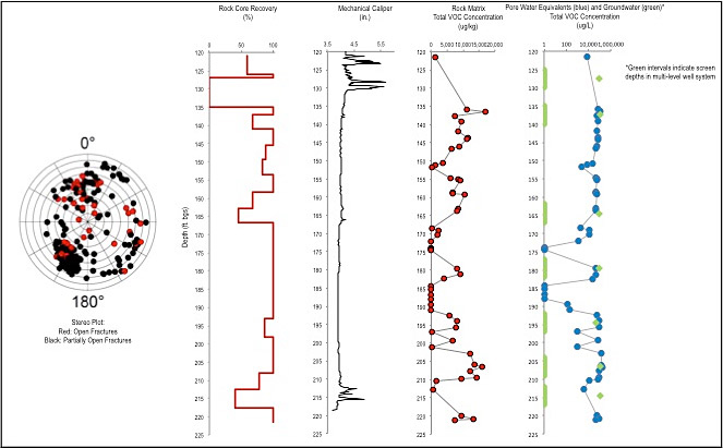
Figure 5-3. Example of a rock matrix analysis, with percent core recovery, mechanical caliper, total VOC, in a multilevel screened well system.

Quantitative analytical results from the rock matrix provide valuable insight into how primary porosity affects contaminant fate and transport at a site. This level of analytical detail may be useful when more detail is required to assess the potential for mass flux and to estimate plume longevity.

Subsequent installation and sampling of groundwater monitoring screens can provide additional information about the mass balance between primary and secondary porosity. For example, suppose groundwater contaminant concentrations from a fracture are notably higher than the calculated pore water concentrations from the adjacent primary porosity. The mass balance ratio provides a line of evidence that contaminants are diffusing into the primary porosity of the rock matrix and presumptive equilibrium has not occurred. These observations indicate a high primary porosity or a contaminant release that occurred in the relatively recent past. In the opposite scenario, the reversed mass balance would indicate that the source has been removed or depleted and concentrations in the secondary porosity are the result of back-diffusion from the primary porosity. When analyzing rock matrix results, note that the pore water concentrations are calculated results based on samples presumed to be representative of the physical properties and carbon content of the rock matrix.

Regardless of the methods used, analyzing the results identifies individual compounds and their concentrations. Speciation along a borehole profile, and laterally across a site, may provide critical information about fate and transport of known and potentially new uncharacterized releases, including from potential off-site sources.

5.7.3 Data Presentation

Compiling the interpreted data into a concise CSM presents challenges unique to each site and the target audience. A well-designed CSM includes a concise summary of interpreted results from the various data collected during the site characterization process. While borehole logs themselves are not considered a complete presentation of a CSM, they provide an essential component of data interpretation that becomes the CSM. These interpretations are typically presented in plan view and as cross-sections. The following examples illustrate these three CSM components (borehole logs, plan view, and cross-sections). Three-dimensional components may also play a useful role and are discussed in more detail in Section 5.7.1 (Data Management) and Chapter 8 (Modeling).

5.7.3.1 Integrated Borehole Logs

Integrated borehole logs combine the multiple logs from the borehole to allow analysis and interpretation of the borehole characteristics, including groundwater and contaminant movement. Interpretation of the data from individual boreholes starts during field logging and is accomplished through the integration and interpretation of the data from the borehole. As discussed in Section 5.7.1, various tools are available to store, assemble, manage, and present data from the various logging tools and to accept user input of other data such as lithologic logs and sample results. These tools can help to arrange logs and other data adjacent to one another and to rescale these data vertically and horizontally, as needed, to display relevant features.

An example of an integrated borehole log is presented in Figure 5-4. This borehole was an open bedrock borehole below the bottom of the steel casing. The bedrock coring information, FLUTe flexible liner transmissivity data, sampling data, and final FLUTe liner construction were plotted at the time of the geophysical logging. This example includes optical and acoustic televiewer logs, lithologic descriptions, various geophysical parameters, HPFM results, and contaminant sampling data.

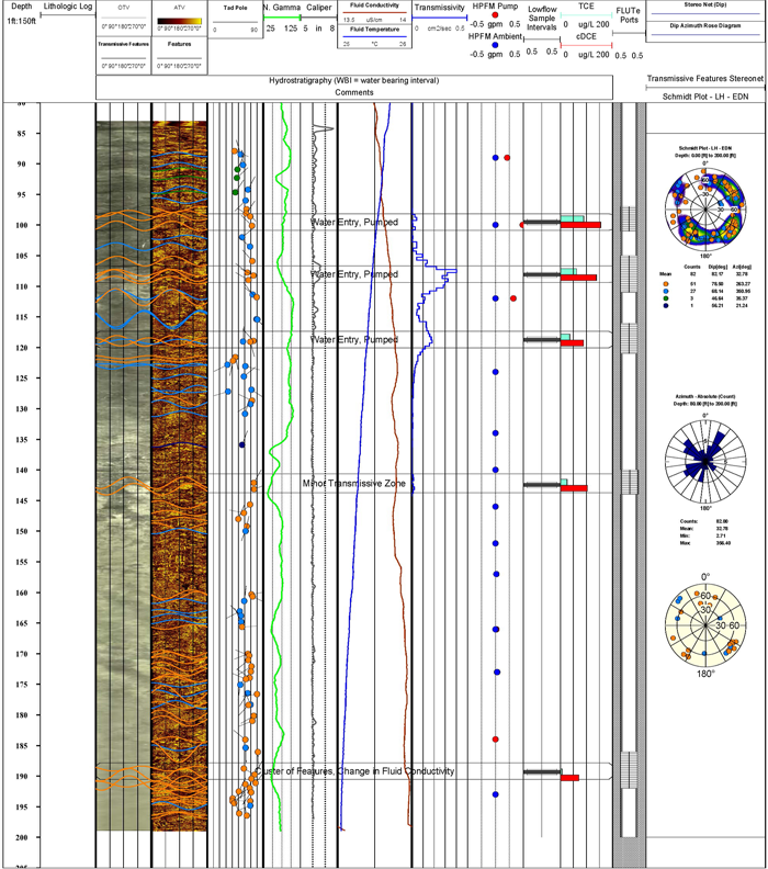
Figure 5‑4. An example of an integrated borehole log.

The raw data for this example were imported into a commercially available software tool and arranged next to one another, from the left to right, on a common vertical scale and datum (for example, top of casing). Typically, rock core and the caliper log are arranged on the left. The televiewer logs are placed next to one another to make it easier to evaluate the same section of borehole in both logs. Likewise, the fluid temperature and fluid conductivity logs are arranged next to, or stacked on, one another so that inflections in both properties can be identified. One advantage of software is that it allows the user to stack logs, such as fluid temperature and conductivity, on top of each other to facilitate data interpretation and to fit more data into the available space. Another critical capability of the software is the log analysis tools built into the software. For example, advanced technology video (ATV) and overlay transport visualization (OTV) data can be used to determine borehole deviation. This feature also allows overlay of a feature log on the ATV and OTV logs and to fit a curve to features, such as fracture, bedding planes, and joints, to determine their dip angle, dip azimuth, and aperture. The feature orientation data can be represented as sinusoidal curves or as tadpole plots. (tadpole plots display the dip angle and azimuth.) The feature log can also be used to create a stereonet diagram and the data can be exported so that all orientation data from all boreholes at the site can be compiled in one stereonet.

The HPFM data were added to the log and used to advance the interpretation of borehole hydraulics, fluid movement, and head distribution. Typically, the pumped and ambient logs are overlaid on one another using a common horizontal scale with zero flow in the middle, negative flow (down flow) to the left, and positive flow (up flow) to the right. This arrangement makes it easier to identify changes in vertical fluid movement between the ambient and pumped logs. The data sets shown on Figure 5-4 were not necessarily all collected at once. Initial logging/profiling activities (such as geophysical logs and televiewer) can be used to define further data collection activities based on the project objectives. As these data are collected, the results can also be incorporated into the software to facilitate data analysis and interpretation of the design of a single screen or multilevel well interval. In this way, each borehole is interpreted individually and then integrated into an overall picture of bedrock hydrogeology of the CSM.

5.7.3.2 Plan View Maps

The purpose of the plan view maps is to depict the lateral component of a 3-D CSM. Multiple maps can be prepared as necessary to encompass regional features but also to offer sufficient detail on the site level. A regional map could be prepared to include lineaments, water shed areas and surface water bodies and high-capacity wells or well fields to orient the reader about general groundwater flow. Increased detail on the site level can include smaller scale plan view maps with focus on contaminant distribution and transport. Illustrating contaminant speciation can help to delineate plumes and their sources, including potential off-site sources upgradient of the site. It is also useful to illustrate groundwater flow direction in the various hydrogeologic units, if available. Because utility trenches are most often dug in overburden and weathered bedrock (saprolite), these trenches are a potentially significant consideration to include in the fractured rock CSM. A utility trench can act as a preferential pathway for source migration or, in the case of leaking utilities, constitute the contaminant source itself. While not comprehensive, Table 5-3 lists various features that should be considered for the various plan view CSM maps. An example of a plan view map as a component of a CSM is shown in Figure 5-5.

Table 5-3. Features that should be included considered for a plan view representing a CSM

Physical Features	Geology	Hydrogeology/Hydrology	Contamination
Monitoring Locations	Topography (surface)	Water sheds	Source Locations
Utility Trenches	Lineaments	Piezometric Contours and Flow Direction	Plume Boundaries and Contaminant Contours
Property Boundaries	Top of Weathered Bedrock Elevation Contours	Extraction Wells in Each Aquifer	Plume Speciation
Human and Ecological Receptors	Faults	Surface Discharge or Recharge Bodies	NAPL Presence
	Top of Competent Bedrock Elevation Contours	Subcropping and Fracture Planes

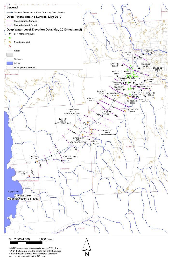
Figure 5-5. Example of a plan view map.

5.7.3.3 Cross-Sections

Geological cross-sections should be positioned and aligned to take maximum advantage of available information and to best present the geology (folds and faults), contaminant transport (groundwater flow direction), and the relationship between them. Relevant well data, however, are commonly situated off the cross-section line and it is useful to project this information onto the section line rather than ignore it. The spatial variability in the geology, groundwater flow, and contaminant distribution warrants increased scrutiny with distance from the cross-section line when projecting data onto a cross-section line. It may not be appropriate to project information such as well data on to a cross-section if there is significant geology or groundwater variation, especially in the direction of the projection (perpendicular to the cross-section line). Use care and professional judgment if these conditions are present.

Intersecting cross-sections, when possible, can help reduce the uncertainty associated with projecting significant amounts of data onto an individual cross-section by constraining the geologic and contaminant transport interpretations in three dimensions and by demonstrating the validity of the CSM. Alternately, cross-sections can be aligned from point to point, with bends in the section. This approach presents other challenges, such as varying apparent dips, and may result in cross-sections that complicate interpretation and visualization of the subsurface.

While not comprehensive, Table 5-4 lists various features that should be considered in the cross-section CSM figures. An example of a cross-section as a component of a CSM is provided in Figure 5-6.

Table 5-4. Features that should be considered for inclusion on a cross section representing a CSM

Physical Features	Geology	Hydrogeology/Hydrology	Contamination
Monitoring Locations	Bedrock Geology	Flow Direction	Source Locations
Utility Trenches	Fracture Orientation	Extraction Wells	Matrix Concentrations
Grade Elevation	Fracture Type	Water Table	Plume Boundaries
Scale and Vertical Exaggeration	Bedding Units (if applicable)	Piezometric Water Levels (if different than water table)	Plume Speciation and Concentration Contours
	Top of competent Bedrock Surface	Hydrogeologic Units and Lower Boundaries	NAPL
	Faults	Surface Discharge and Recharge bodies
	Top of weathered bedrock	Receptors
		Preferential Migration Pathways
		Interconnectivity

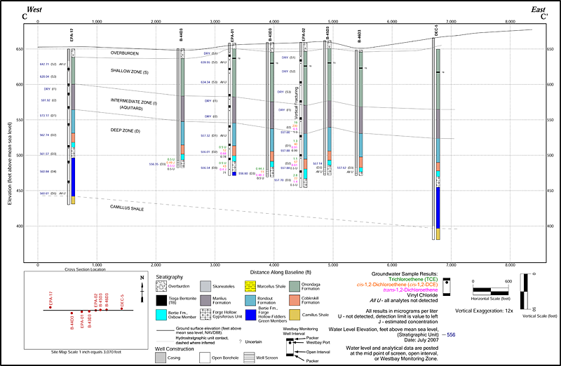
Figure 5-6. Example of a cross section used within a CSM